Ann Optax Flax#
ANN, Flax, Optax#
So far, you’ve seen how to define a model using jax, train the model, do backpropagation, and test it. Let’s take it a bit further. In this notebook we’ll be writing a simple ANN to classify penguin species using the palmers penguin dataset.
Since it’s the first notebook on something NN, it’ll be a good opportunity to introduce the Neural Net library in the Jax ecosystem, Flax. Also, like the linear regression example, we’ll have to update the model parameters during backpropagation, for which there is also a library, Optax. In this notebook, I’ll show you how to use both with a simple classifier.
Let’s load the data and process it to get started. (apparently the main focus of this notebook is to show you the ANN and not how you can load data, so, I’m going to short circuit the data related process a bit)
Data#
# setting up device backend for apple silicon (mps)
# if you have it that is.

from utils import setup_backend, log_device

setup_backend()
log_device()
2026-05-07 19:28:54.684 | INFO     | utils.device:setup_backend:24 - Setting up JAX to use the `mps` backend.
2026-05-07 19:28:54.685 | SUCCESS  | utils.device:setup_backend:26 - JAX Platform set to use the `mps` backend.
Platform 'mps' is experimental and not all JAX functionality may be correctly supported!
2026-05-07 19:28:54.816 | INFO     | utils.device:log_device:14 - XLA DEVICE: mps
import numpy as np
import pandas as pd
from palmerpenguins import load_penguins
import jax
import jax.numpy as jnp

from tqdm.auto import tqdm
from sklearn import preprocessing


def load_data():
    penguins = load_penguins() # penguins is a dataframe
    penguins = penguins.dropna() # type: ignore

    # print the head of the dataframe to give some view
    print(penguins.head()) # type: ignore

    # collect the feature columns
    feature_columns = ['bill_length_mm', 'bill_depth_mm', 'flipper_length_mm', 'body_mass_g']
    # classification target
    target_column = "species"

    # features and targets
    features = penguins[feature_columns].values  # type: ignore
    targets = penguins[target_column].values  # type: ignore

    # but here's a catch
    # the targets are categorical, so we have two two options here
    # one hot encode them, or, assign a numeric value to them and keep a dictionary
    # with the target label to int mapping
    # the second approach is easier xD

    target_ids_dict = dict()
    unique_target_labels = set(targets)
    _id = 0

    for ul in unique_target_labels:
        target_ids_dict[ul] = _id
        _id += 1

    # convert target labels to integers using the same dict
    def convert_label_to_ids(targets, id_dict):
        converted_targets = np.zeros(shape=(len(targets, )), dtype=np.int32)
        for idx, target in tqdm(enumerate(targets)):
            converted_targets[idx] = id_dict[target]

        return converted_targets

    targets_converted = convert_label_to_ids(
        targets=targets, id_dict=target_ids_dict)

    assert features.shape[0] == targets_converted.shape[0]

    # the features from the dataset are not normalised and
    # this can cause probblems during training, such as
    # gradients getting stuck in a local minima
    # there's a lot of literature which talks about the
    # necessity of normalisation, this is a good starter
    # https://machinelearningmastery.com/how-to-improve-neural-network-stability-and-modeling-performance-with-data-scaling/

    features_norm = preprocessing.normalize(features, norm="l2")


    return (features_norm, targets_converted)


X, y = load_data()
print(X.shape) # type: ignore
print(y.shape) # type: ignore
  species     island  bill_length_mm  bill_depth_mm  flipper_length_mm  \
0  Adelie  Torgersen            39.1           18.7              181.0
1  Adelie  Torgersen            39.5           17.4              186.0
2  Adelie  Torgersen            40.3           18.0              195.0
4  Adelie  Torgersen            36.7           19.3              193.0
5  Adelie  Torgersen            39.3           20.6              190.0

   body_mass_g     sex  year
0       3750.0    male  2007
1       3800.0  female  2007
2       3250.0  female  2007
4       3450.0  female  2007
5       3650.0    male  2007
(333, 4)
(333,)
Okay splendid. Now to create the data split and also convert these numpy arrays to jax arrays.
from sklearn.model_selection import train_test_split

features_train, features_test, targets_train, targets_test = train_test_split(
    X, y, test_size=0.3, random_state=42)


features_train = jnp.array(features_train)
features_test = jnp.array(features_test)
targets_train = jnp.array(targets_train)
targets_test = jnp.array(targets_test)


print(f"Train Size : {features_train.shape[0]}")
print(f"Test Size: {features_test.shape[0]}")
Train Size : 233
Test Size: 100
ANN#
This is going to be a 2 layer ANN with Leaky ReLU activation, 3 target classes and cross entropy as the loss function.
PRNG#
# old ritual of generating prngs
key = jax.random.key(3047)
ANN definition#
In Flax, flax.linen provides all the necessary bells and whistles to implement neural networks. If you’re coming from pytorch, this is equivalent to torch.nn.
Another intresting thing about Flax is that, despite Jax being functional, Flax does make use of classes (as PyTorch does!). Let’s see the class definition.
import flax.linen as nn


class PenguinFinder(nn.Module):
    in_dim: int
    hidden_dim: int
    out_dim: int

    def setup(self):
        # layer definition goes here
        self.layer1 = nn.Dense(features=self.in_dim)
        self.hidden = nn.Dense(features=self.hidden_dim)
        self.layer2 = nn.Dense(features=self.out_dim)

    def __call__(self, x):
        out = self.layer1(x)
        # out = nn.relu(out)

        out = self.hidden(out)
        # out = nn.relu(out)

        out = self.layer2(out)
        out = nn.leaky_relu(out)

        # apply softmax to convert to
        # probability distribution
        logits = jax.nn.softmax(out)

        return logits
Let’s take a look at the class definition here. First we declare the variables / hyperparameters to init the model as static python vars. Next we have a setup method which defines the layers in the NN. The __call__ method is similar to what you see as forward in Pytorch, it applies all the layer operations on your data.
The setup method comes in handy if you have to modify the default behavior of some linen class or want to define your own custom layers. If this is not the case (you want to use linen classes as they are), you can reduce the code by getting rid of setup and using compact. The class definition will then look like this
class PenguinFinder(nn.Module):
    in_dim: int
    hidden_dim: int
    out_dim: int

    @nn.compact
    def __call__(self, x):
        out = nn.Dense(features=self.in_dim)(x)
        out = nn.Dense(features=self.hidden_dim)(out)
        out = nn.Dense(features=self.out_dim)(out)
        out = nn.leaky_relu(out)

        # apply softmax
        logits = jax.nn.softmax(out)

        return logits
# init model
model = PenguinFinder(in_dim=4, hidden_dim=4, out_dim=3)
params from a linen module are returned as a Frozen dict, which is immutable. During training, when we won’t be updating the params in place, rather Flax has some nifty trick with training state which we’ll see pretty soon.
# model params
# requires a PRNG key and an array with the same shape of unbatched input
params = model.init(key, features_train[0])
# example forward pass
model.apply(params, features_train[0])
Array([0.33331168, 0.333406 , 0.3332823 ], dtype=float32)
Loss function and grad#
The formal definition of cross entropy loss for a multiclass classification is this: $\( ce = -\sum_{c=1}^My_{t}\log(p_{t}) \)$
where, \(t\) stands for the correct class
\(y_t\) is the correct label and \(p_t\) is what a model predicted for \(t\)
There is a nifty trick to it if you represent your classes with int ids as I have done above. The ids start from 0, so you can basically treat them as indexes. Using this, the cross entropy for an instance basically becomes
This trick works fine for single dimension multi class probabilities. I have never verified it outside course assignments or simple experiments. Then again, this notebook is just here to show you how jax works. In practice, it’ll be buckwild to write everything from scratch. Don’t violate the DRY principle!
# loss function
# for a single instance
# will vmap for batches

@jax.jit
def cross_entropy(params, x, y):
    # forward pass .....
    logits = model.apply(params, x)

    return -jnp.log(logits[y]) # type: ignore


cross_entropy(params, features_train[0], targets_train[0])
Array(1.0986773, dtype=float32)
@jax.jit
def calculate_loss(params, x_batched, y_batched):
    batch_loss = jax.vmap(cross_entropy, in_axes=(None, 0, 0))(params, x_batched, y_batched)
    return jnp.mean(batch_loss)


calculate_loss(params, features_train, targets_train)
Array(1.0986663, dtype=float32)
Optimisation#
This is where we introduce Optax. For this notebook, I’m using the Adam optimiser.
There are other optimizers in Optax which you can use: https://optax.readthedocs.io/en/latest/api.html
Also, more on Adam: https://arxiv.org/abs/1412.6980
import optax

optimiser = optax.adam(learning_rate=0.01)
loss_grad_fn = jax.value_and_grad(calculate_loss)
Flax Train state#
Okay so we’ve an optimiser but we need to tell it how it should be updating the parameters. We can do it using optax, go through the frozen dict (after making it immutable and froze it agian) but that’s too much hassle and opens up more avenues for user error. Instead we’ll be using train_state in Flax.
from flax.training import train_state

model_state = train_state.TrainState.create(
    apply_fn=model.apply, # the forward function
    params=params,
    tx=optimiser
)
During training, all we have to do is update this model state, and Flax will do the rest for us. (It’ll be easier to understand the whole process if we consider params as states for models.)
Train-ing#
Finally! Der Zug ist da! (Oh wait……….no, it’s late again.)
# batched
@jax.jit
def train_step(state, xs, ys):
    loss_value, grads = loss_grad_fn(state.params, xs, ys)
    state = state.apply_gradients(grads=grads)
    return loss_value, state
from tqdm.auto import trange


def train(state, xs, ys, epochs, log_every_n_step):
    losses = list() # keeps track of losses every n steps
    steps = list()

    step_count = 0

    for e in trange(epochs):
        loss, state = train_step(state, xs, ys)
        if step_count % log_every_n_step == 0:
            losses.append(loss)
            steps.append(step_count)

            print(f"Epoch = {e + 1} / {epochs} \t :: Train Loss = {loss}")
        step_count += 1

    return state, losses, steps
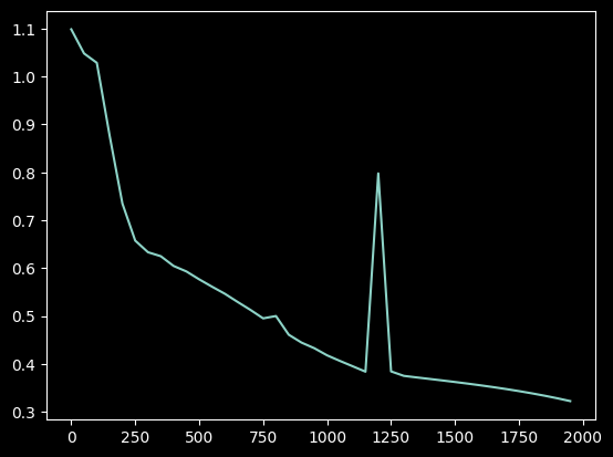
trained_model_state, losses, steps = train(model_state, features_train, targets_train, 2000, 50)
Epoch = 1 / 2000 	 :: Train Loss = 1.0986663103103638
Epoch = 51 / 2000 	 :: Train Loss = 1.0482356548309326
Epoch = 101 / 2000 	 :: Train Loss = 1.0285781621932983
Epoch = 151 / 2000 	 :: Train Loss = 0.8766480684280396
Epoch = 201 / 2000 	 :: Train Loss = 0.734576404094696
Epoch = 251 / 2000 	 :: Train Loss = 0.6573436260223389
Epoch = 301 / 2000 	 :: Train Loss = 0.6330532431602478
Epoch = 351 / 2000 	 :: Train Loss = 0.6247238516807556
Epoch = 401 / 2000 	 :: Train Loss = 0.6043933629989624
Epoch = 451 / 2000 	 :: Train Loss = 0.5929273366928101
Epoch = 501 / 2000 	 :: Train Loss = 0.5764503479003906
Epoch = 551 / 2000 	 :: Train Loss = 0.5611416697502136
Epoch = 601 / 2000 	 :: Train Loss = 0.5464057326316833
Epoch = 651 / 2000 	 :: Train Loss = 0.5293152332305908
Epoch = 701 / 2000 	 :: Train Loss = 0.5127198100090027
Epoch = 751 / 2000 	 :: Train Loss = 0.4949222803115845
Epoch = 801 / 2000 	 :: Train Loss = 0.4997834265232086
Epoch = 851 / 2000 	 :: Train Loss = 0.4608038365840912
Epoch = 901 / 2000 	 :: Train Loss = 0.4443221986293793
Epoch = 951 / 2000 	 :: Train Loss = 0.43258658051490784
Epoch = 1001 / 2000 	 :: Train Loss = 0.41770514845848083
Epoch = 1051 / 2000 	 :: Train Loss = 0.4060603380203247
Epoch = 1101 / 2000 	 :: Train Loss = 0.3948742747306824
Epoch = 1151 / 2000 	 :: Train Loss = 0.38360628485679626
Epoch = 1201 / 2000 	 :: Train Loss = 0.7977051734924316
Epoch = 1251 / 2000 	 :: Train Loss = 0.3841603100299835
Epoch = 1301 / 2000 	 :: Train Loss = 0.37480399012565613
Epoch = 1351 / 2000 	 :: Train Loss = 0.3715763986110687
Epoch = 1401 / 2000 	 :: Train Loss = 0.3684562146663666
Epoch = 1451 / 2000 	 :: Train Loss = 0.36528506875038147
Epoch = 1501 / 2000 	 :: Train Loss = 0.3620149791240692
Epoch = 1551 / 2000 	 :: Train Loss = 0.3586122691631317
Epoch = 1601 / 2000 	 :: Train Loss = 0.3550443649291992
Epoch = 1651 / 2000 	 :: Train Loss = 0.3512757122516632
Epoch = 1701 / 2000 	 :: Train Loss = 0.3472684323787689
Epoch = 1751 / 2000 	 :: Train Loss = 0.34297990798950195
Epoch = 1801 / 2000 	 :: Train Loss = 0.33836519718170166
Epoch = 1851 / 2000 	 :: Train Loss = 0.33338508009910583
Epoch = 1901 / 2000 	 :: Train Loss = 0.3279927670955658
Epoch = 1951 / 2000 	 :: Train Loss = 0.32214710116386414
%matplotlib inline
import matplotlib.pyplot as plt
import seaborn as sns


sns.lineplot(x=np.array(steps), y=np.array(losses))
plt.show()
Evaluation#
@jax.jit
def test_step(state, x):
    logits = model.apply(state.params, x)
    out = jnp.argmax(logits, axis=-1)

    return out


@jax.jit
def test(state, xs):
    return jax.vmap(test_step, in_axes=(None, 0))(state, xs)
predictions = test(trained_model_state, features_test)
from sklearn.metrics import classification_report

report = classification_report(y_pred=predictions, y_true=targets_test)
print(report)
              precision    recall  f1-score   support

           0       0.72      0.92      0.81        48
           1       0.60      0.26      0.36        23
           2       1.00      1.00      1.00        29

    accuracy                           0.79       100
   macro avg       0.77      0.73      0.72       100
weighted avg       0.77      0.79      0.76       100
A fun little experiment#
Comment out all the @jax.jit annotations, restart the jupyter server and run all the cells again. Check how long it takes to train the network.
tsk tsk ;)